How much of a good backtest is luck?
112 parameterizations of four textbook strategy families were
backtested on the 49 Kenneth French industry portfolios (1969-07 to
2026-08, 686 months, 10 bps costs,
10.0% volatility target). The best one is then put through the standard
overfitting diagnostics. All numbers on this page are read from
results/summary.json.
The selected strategy
xsmom(lookback=12,skip=0,quantile=0.2)|vol12 has the highest full-sample net Sharpe ratio,
0.68 (95% block-bootstrap CI 0.41 to 0.95; the interval treats this
trial as if it had been fixed in advance and does not account for having picked it from
112). Its Sharpe was 0.90 before
1998-02 and 0.46 after.
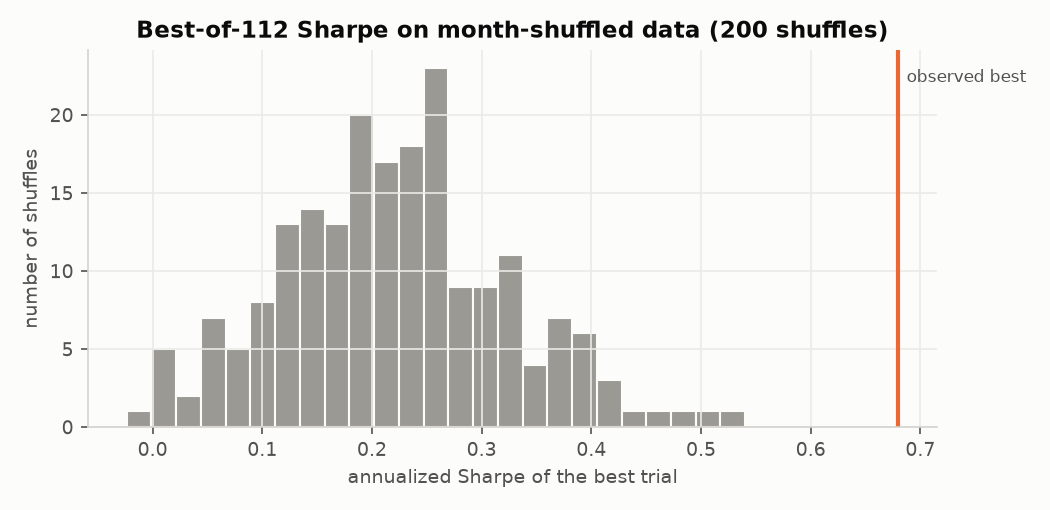
On month-shuffled data the best of the same grid averaged 0.22 (max 0.54, p = 0.005). Shuffling also removes the volatility clustering that volatility targeting uses, so the same test was repeated without volatility targeting: the selected signal then has a Sharpe of 0.52, the best of 56 unscaled signals 0.52, against a shuffled best-of-grid mean of 0.20 (p = 0.005).
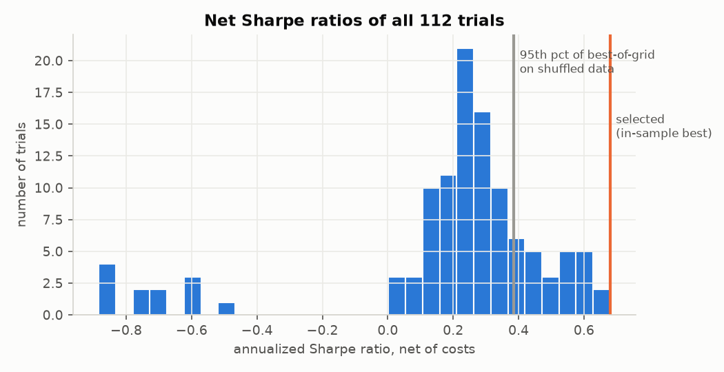
The Deflated Sharpe Ratio compares the selected Sharpe with the expected best of N skill-less trials, which depends on N and on the variance of Sharpe ratios across trials. Sign-aligning flips families whose median Sharpe is negative (reversal); the effective N is the participation ratio of the eigenvalues of the trial correlation matrix.
| Var[SR] and N used | N | Std of SR | E[max SR] | DSR |
|---|---|---|---|---|
| Raw trial Sharpes (paper recipe) | 112.0 | 0.35 | 0.90 | 0.049 |
| Sign-aligned families | 112.0 | 0.20 | 0.51 | 0.893 |
| Sign-aligned, effective N | 3.1 | 0.20 | 0.18 | 1.000 |
| No-signal variance from shuffles | 112.0 | 0.13 | 0.34 | 0.994 |
| Trials assumed (N), sign-aligned Var[SR] | DSR |
|---|---|
| 1 | 1.000 |
| 4 | 1.000 |
| 10 | 0.997 |
| 30 | 0.976 |
| 112 | 0.893 |
| Cost per unit turnover | Sharpe |
|---|---|
| 0 bps | 0.76 |
| 10 bps | 0.68 |
| 25 bps | 0.56 |
| 50 bps | 0.37 |
Probability of Backtest Overfitting
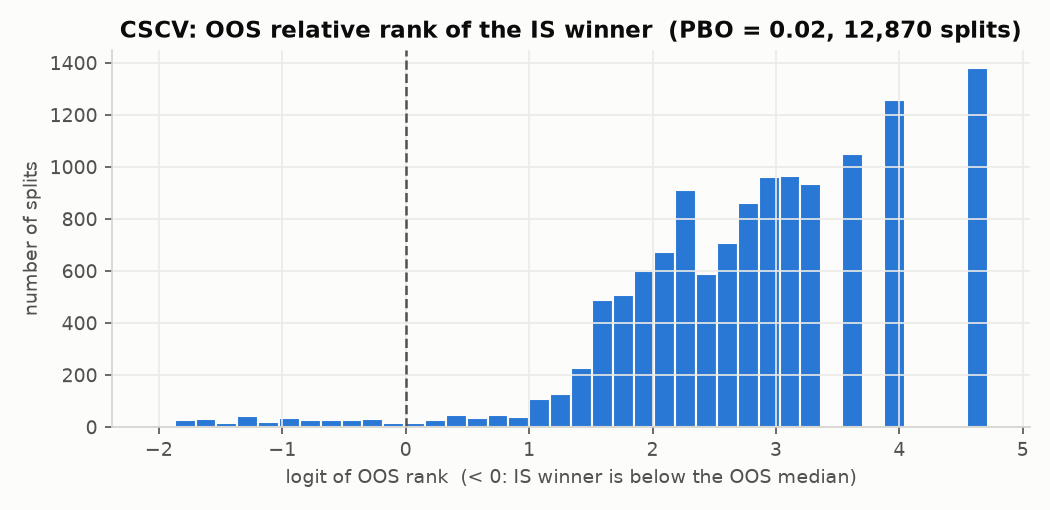
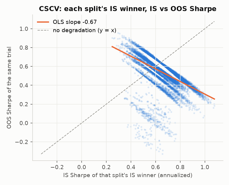
CSCV splits the 672 months into 16 blocks and evaluates all 12,870 half/half splits. The in-sample winner lands below the out-of-sample median in 2.4% of splits and loses money out of sample in 0.9%. Median Sharpe of the winner: 0.66 in sample, 0.54 out of sample. Across splits, the OOS Sharpe of the winner falls as its IS Sharpe rises (OLS slope -0.67); part of this is mechanical, because the two halves are complements of one fixed sample.
| Family | Trials | Best Sharpe | Median Sharpe | PBO |
|---|---|---|---|---|
| xsmom | 48 | 0.68 | 0.38 | 0.02 |
| tsmom | 14 | 0.39 | 0.21 | 0.32 |
| ma_cross | 38 | 0.36 | 0.22 | 0.34 |
| reversal | 12 | -0.52 | -0.74 | 0.01 |
Walk-forward selection
Every 12 months, pick the trial with the best Sharpe over the trailing 120 months and hold it. Over 48 windows this chose 18 distinct trials.
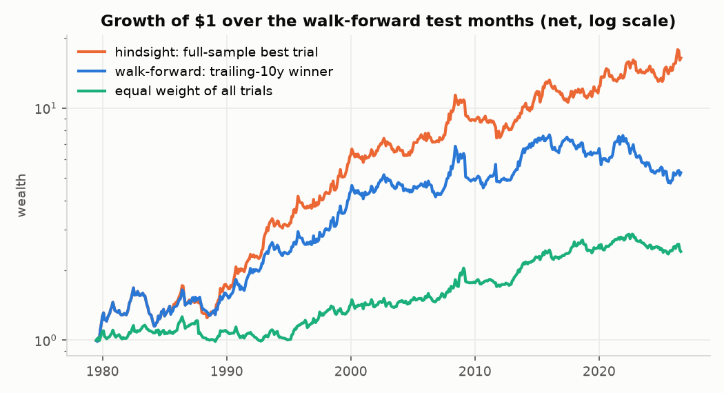
| Series (same months) | Sharpe | Ann. return |
|---|---|---|
| Walk-forward OOS | 0.36 | 4.2% |
| Hindsight best, same months | 0.57 | 6.6% |
| Equal weight of all trials | 0.30 | 2.1% |
Walk-forward OOS Sharpe 95% bootstrap CI: 0.05 to 0.68.
Factor-adjusted alpha
OLS on Fama-French factors with Newey-West standard errors.
| Series | Model | Alpha (ann.) | t (NW) | Lags |
|---|---|---|---|---|
| Selected (hindsight) | FF3 | 9.6% | 5.66 | 6 |
| Selected (hindsight) | FF5 | 9.5% | 5.17 | 6 |
| Walk-forward OOS | FF3 | 4.4% | 2.46 | 5 |
| Walk-forward OOS | FF5 | 3.8% | 2.04 | 5 |
Top 10 trials
| Trial | Sharpe | Ann. ret | Ann. vol | Max DD | Turnover/yr |
|---|---|---|---|---|---|
| xsmom(lookback=12,skip=0,quantile=0.2)|vol12 | 0.68 | 8.1% | 11.9% | -34.7% | 9.4 |
| xsmom(lookback=12,skip=0,quantile=0.3)|vol12 | 0.64 | 7.6% | 11.9% | -31.0% | 9.8 |
| xsmom(lookback=12,skip=1,quantile=0.2)|vol12 | 0.63 | 7.4% | 11.8% | -24.5% | 9.5 |
| xsmom(lookback=12,skip=0,quantile=0.2)|vol36 | 0.62 | 7.1% | 11.4% | -33.0% | 7.4 |
| xsmom(lookback=12,skip=1,quantile=0.3)|vol12 | 0.61 | 7.3% | 11.8% | -24.6% | 10.2 |
| xsmom(lookback=12,skip=0,quantile=0.1)|vol12 | 0.60 | 7.1% | 11.9% | -29.9% | 7.9 |
| xsmom(lookback=12,skip=0,quantile=0.3)|vol36 | 0.58 | 6.6% | 11.3% | -27.6% | 7.7 |
| xsmom(lookback=12,skip=1,quantile=0.2)|vol36 | 0.56 | 6.3% | 11.2% | -31.4% | 7.6 |
| xsmom(lookback=12,skip=0,quantile=0.1)|vol36 | 0.56 | 6.3% | 11.2% | -30.2% | 6.4 |
| xsmom(lookback=9,skip=0,quantile=0.2)|vol12 | 0.56 | 6.7% | 12.0% | -29.5% | 10.9 |
Data and methods
- Data: Kenneth R. French Data Library, https://mba.tuck.dartmouth.edu/pages/faculty/ken.french/data_library.html (This file was created using the 202608 CRSP database.). Raw files are not redistributed; the repository contains a download script.
- Signals use information up to month t and are traded in month t+1; costs are charged per unit of turnover; positions are scaled to a volatility target using trailing realized volatility.
- Bailey, Borwein, López de Prado, Zhu (2017), The Probability of Backtest Overfitting, Journal of Computational Finance 20(4). Bailey & López de Prado (2014), The Deflated Sharpe Ratio.